Interview Preparation: Design A System To Get TopK Elements At Scale
Finding Heavy Hitters

Hello there 👋 ! We are growing fast and are now at 2000+ subscribers 💪 💪. Thank you for your love and support ❤️ ❤️. I am enjoying it, I hope you are enjoying it too!
A quick recap. In the last three newsletters, we looked at the design of a distributed cache, the lessons from Netflix’s notification service, the design of a scalable notification service, and the design of a scalable search engine. In this newsletter, I discuss the design of a distributed cache. I hope you enjoy reading this one. You can use this for your interview preparation.
In this blog post, I will discuss the problem of finding the top k hits within a given period. To relate to the problem better, let us imagine that you are building a Google-like search engine, and you need to be able to find the top-k queries within the last one day.
I have also combined all the blogs in a free sample e-book for anyone to download.
Note: I would call out that I have used this YouTube video for writing most of this blog post. I liked how The System Design Interview channel is built - although it has been dormant for some time now.
Understanding The Real World UseCase
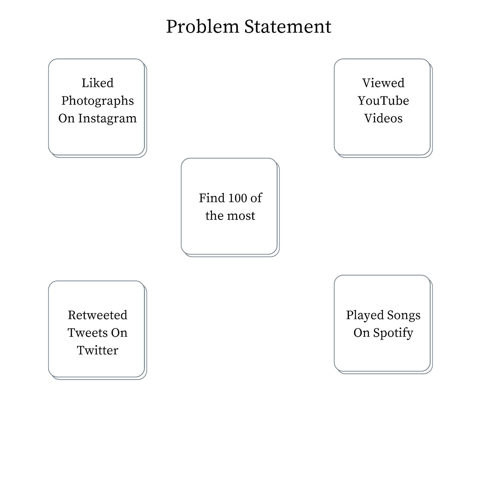
Figure 1 depicts some of the use cases in the real world that require the system to solve the problem of finding the top-K heavy hitters. Let us say that you log in to your Instagram account. The homepage shows you the top 100 trending pictures or accounts on Instagram. The problem is solved in the background using a similar system (that we will end up designing as a part of this chapter). Other examples include the most retweeted tweets in the last twenty-four hours, the most played song on Spotify, or the most viewed video on YouTube.
Understanding Scale
The most important principle of solving a system design problem is to understand the constraints of the system. The solution one can design depends heavily on the scale of the inputs, the requirements of the outputs, and the resources available to build the system. For the scope of this problem we should assume the following:
The system can contain billions of items;
Each item may have a size of 10 MBs;
The output is required within tens of seconds;
The system can deploy thousands of compute nodes; and
The system can have infinite storage space.
Can We Use MapReduce?
It may be apparent that this problem needs to be solved in real-time. You may end up discussing this with the interviewee to get a sense of whether they want to solve this in real-time or not. If the requirement is to get the search results within a few seconds then it requires a real-time solution. Solutions involving MapReduce may be out of the window as they tend to batch updates and require a longer timeframe. MapReduce persists intermediate data on disks and therefore may not be able to return results within a small bounded time interval and thus may not qualify as real-time.
Functional Requirements
We want our system to return the list of K most frequent items over a predefined time interval.
topk (K, startTime, endTime)
Non-Functional Requirements
As discussed in our previous blog posts, the system should adhere to specific non-functional requirements. Some of these requirements are as follows:
Scalable - The system should scale with an increasing amount of data ingested.
Available - The system should survive hardware and software failures, i.e., no single point of failure.
Performant - The system should be able to return the top 100 list of items within hundreds of milliseconds.
Accurate - The system may return an approximate solution. With data sampling, we can calculate an approximate list. This may be sufficient for specific use-cases such as approximate analysis. We would need to design a system that can return the topK results.
Exploring The Solution Space
First, we start with the basics using a first-principles approach and then work towards the more complex solutions. It is generally good to start with a simple design and then work towards more complex designs. Why does this matter? It helps the interviewer understand your thought process and shows them that you are a systematic thinker. I adopt this approach whenever I am interviewing or discussing a problem in System Design.
Solution #I: Hash table, single host
For the sake of this solution, let us make the following assumptions:
Assumption #1:
Let us also assume that all the data can fit on single server memory.
Assumption #2:
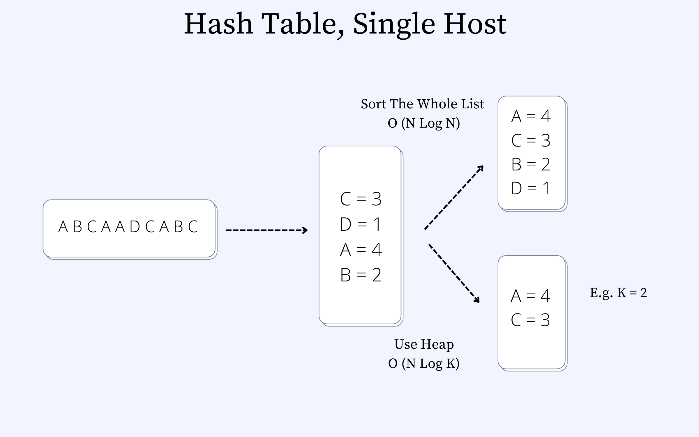
Let us assume a collection of video events where each of the letters in the figure below represents a video. So, the letter “A” represents Video 1, “B” represents Video B, etc. We can imagine this as a video streaming service such as YouTube or Netflix.
We can sort the list or use a heap. The heap approach is faster. The time complexity of sorting is O(N log N), and that with the heap is O(N log K), where N is the total number of unique videos and K represents the total number of videos to be returned.
Drawbacks:
The solution is not scalable. If the rate at which the elements hit the single host increases, the host may quickly become bottlenecked on the CPU. Let us explore an improvement to this solution by introducing a load balancer.
Solution #2: Hash Table, Multiple Hosts, Load-Balancing
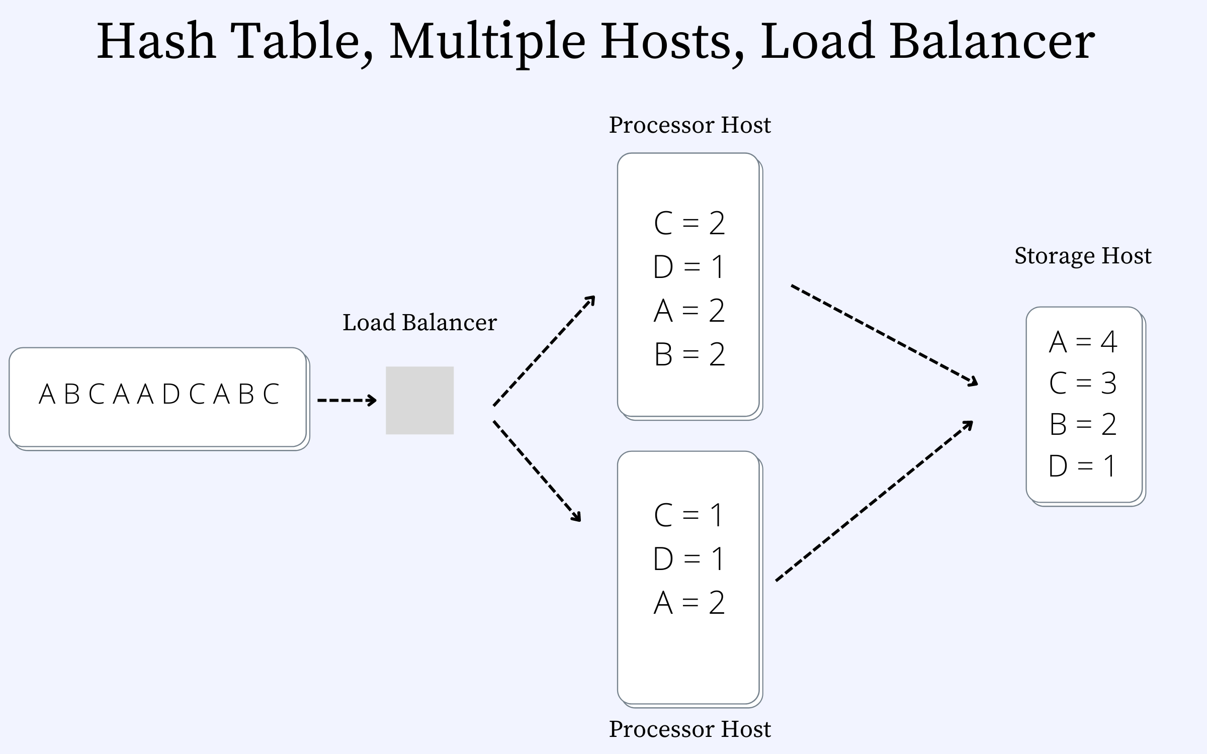
Figure 3 shows the updated design with a load-balancer and the processing now distributed between two different hosts. The solution works a bit better now. The total throughput of the system has increased now. However, the system can still get bound by memory. Typically, YouTube may end up having billions of videos. Storing these into a single host machine may not be feasible as the server may start to run into OOM (Out-Of-Memory) issues.
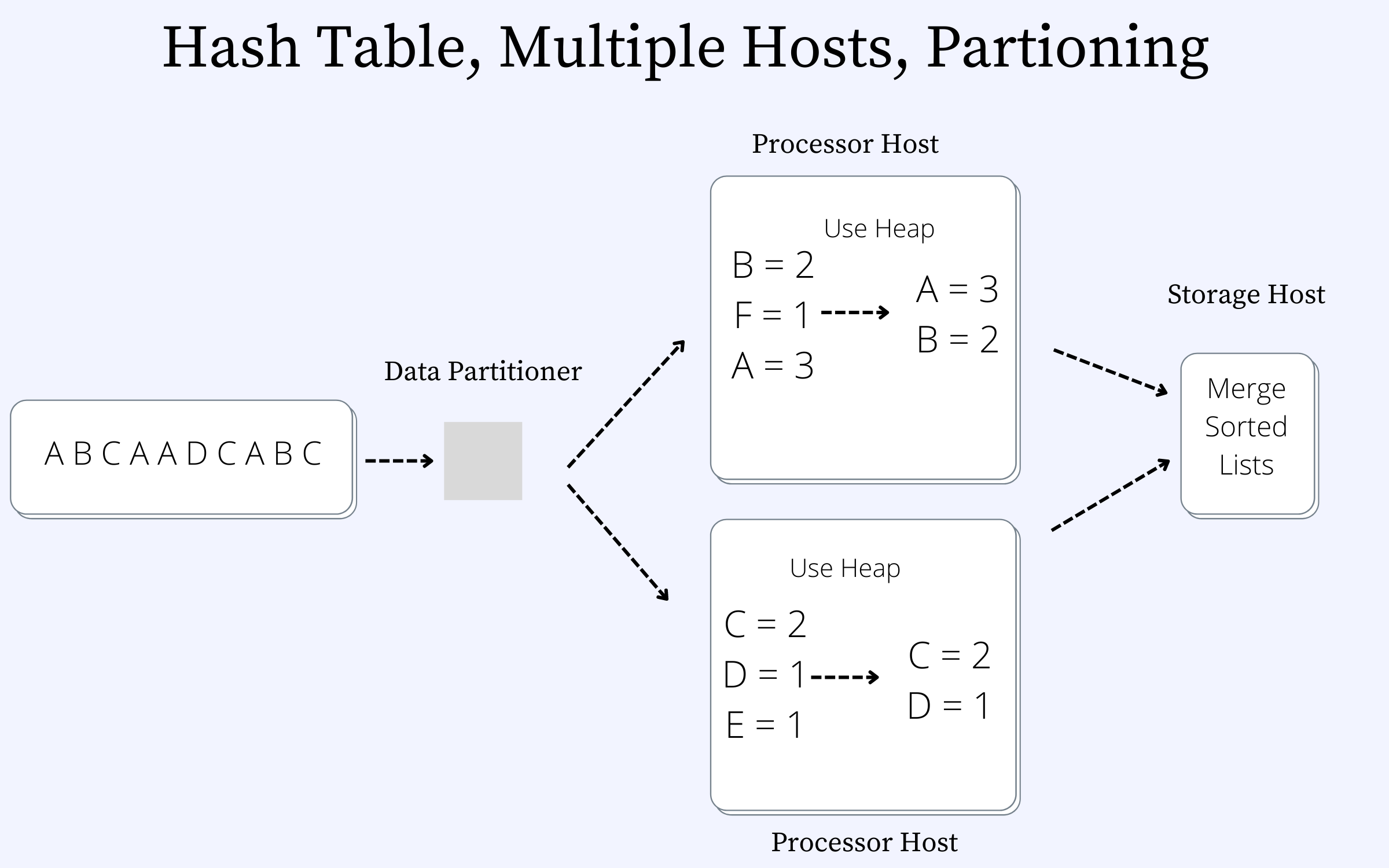
Solution #3: Hash Table, Multiple Hosts, Partitioning
Figure 4 shows a data partitioner in front of the processor hosts. Each processor contains a subset of the videos. Each of the processor hosts contains its list of top k heavy hitters. We will need to merge the two sorted lists to get the final list. It is important to note that we cannot pass the entire hash table list to the storage host.
Complexities Involved
While the design with data partitioning makes the system extremely scalable, we still need to deal with certain complexities in building the architecture. Let us go through these ones by one and discuss them in detail.
Complexity #1: Data Replication
The first problem that the system needs to deal with is to ensure that the data is replicated across the different nodes. Let us go through and revise what data replication is first. (I covered some of the fundamentals of system design in this blog post, in case you are interested in revisiting it). Data replication is a method of copying data to ensure that all information stays identical in real-time between all data resources. Think of database replication as the net that catches your information and keeps it falling through the cracks and getting lost. Why is data replication required? Data replication is required to ensure that the system does not lose data in case one of the processor hosts shuts down during the course of the system’s lifetime. Generally, a replication factor of 3 is used in real-world systems. This means that any dataset is kept at a primary host and copied to two more hosts on the network. It is worth noting that the probability of simultaneous failure of three different nodes is close to zero.
Complexity #2: Rebalancing
Computer machines tend to be faulty and can often crash. What should the ideal response of a system be if one of the machines crashes? What if we want to add more nodes to the cluster to get a higher level of parallelism from the system? The answer to those questions is building a system that can rebalance itself. In the following subsection, let us discuss the two scenarios where a node is added to the system and when a node is deleted from the system.
Case #1: Addition of a new node.
If a new node is added to the cluster, we need to ensure that data from existing nodes is divided and moved to the new node. This is achieved by keeping the metadata for the cluster in the Data Partitioner. What does the metadata contain? Ideally, the metadata contains the following:
An identifier for each processor host in the cluster;
The range of data contained on each of the processor hosts;
The data are replicated copies and locations on the different processor hosts.
When a new node is added to the system, the metadata is updated to reflect data movement to the new node.
Case #2: Deletion of a node from a cluster.
If a node is deleted from the cluster, the data that resides on the node needs to move to other nodes. The partitioning node updates the metadata and sends a request to the new nodes so that they query the old nodes and receive the data from them.
Now, we may wonder what complexity underlines the situations above. There are many tricky edge-cases and situations which may arise. Some of the situations that can cause the system to fail are as follows:
Network partition in case data was being moved during rebalancing.
A node goes out of memory or disk and cannot receive a different dataset.
The partitioner node goes down, and the metadata becomes inconsistent with the cluster state.
We will talk about some of these situations in upcoming blog posts.
Complexity #3: Dealing With Hot Partitioning
The last of the complexities that I want to talk about is the problem of hot partitioning. The distribution of access usually follows a Zipfian curve or a heavy-tailed distribution curve. For example, this tweet by Ellen Degeneres has been retweeted more than 3 million times or the video stream of an IPL final on Hotstar, which had 18.6 Million concurrent connections. During the Indian Premier League (IPL) final match between the Chennai Super Kings and Mumbai Indians, the record was set. Some amazing numbers! However, the issue with such access patterns tends to be that one of the nodes on the system would become heavily loaded and would become a laggard in the system. The system's overall performance is dependent on the slowest link in the overall chain. There are several mechanisms to deal with hot-partitioning. We will discuss this in a future blog post.
Merge N Sorted Lists Algorithm
Once the data has been partitioned on each of the individual processor nodes, it is sorted using a heap and then merged into the Storage Processor. An n-way merge algorithm is used to merge the sorted lists. A good resource for learning the algorithm is here. I have kept the algorithm design out of the scope of this discussion deliberately.
Drawbacks:
The solution that we have worked for is a set of videos considering a bounded time interval. However, in a real-world scenario, keeping track of all the videos visited within a day on YouTube may not be entirely feasible.
Data Structure
Before we go further, let us first think through the possible data structures that can help us achieve keeping an approximate counter within a bounded memory space.
Count-Min Sketch
Count-min Sketch is a probabilistic data structure meaning that the frequencies computed may not be accurate but will have some bounded errors. The goal of the basic version of the count–min sketch is to consume a stream of events, one at a time, and count the frequency of the different types of events in the stream. Let us first take a deep dive into the design of the count-min sketch data structure.
How is the data structure designed?
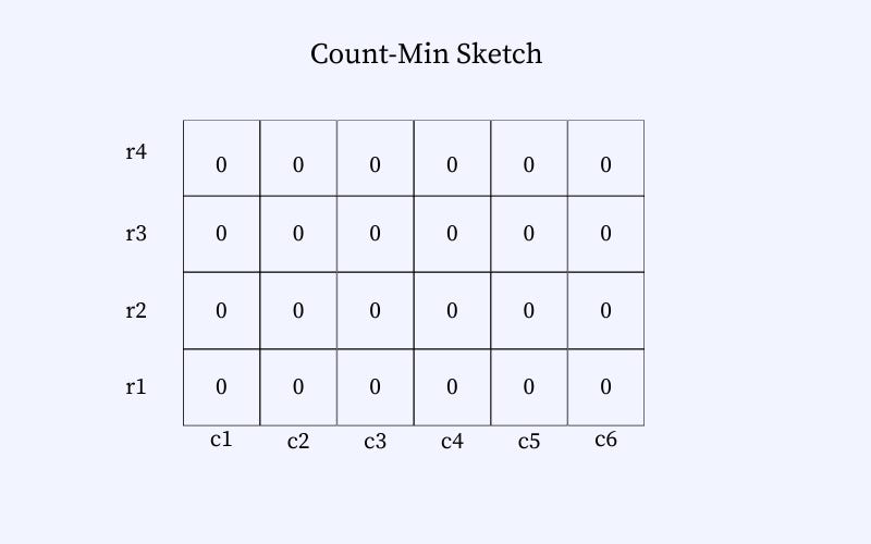
The Min-Sketch counter has a pre-defined memory allocated. We can imagine it as a 2D grid. Each cell holds an integer, indicating the number of times an element hashes to the cell. The initial value of each of the cells is 0. The figure below represents a representation of an empty count-min sketch data structure.
A sample workflow.
Let us go through an example to understand the data structure. We need to store the counts of the following inputs: “A-A-B-C.” We go through the figures below to understand how the data structure is updated and then how we retrieve the count corresponding to each of the elements (i.e., A, B, and C). Note that the counts corresponding to each element remain approximate when using this data structure.
The figure below shows an empty Count-min Sketch data structure. The data structure consists of a set of columns and rows. The size of the data structure is fixed. The size of the hash function depends on the correctness that is desired from the data structure. A higher accuracy requires a larger memory footprint of the data structure.
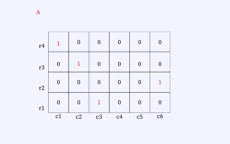
In the figure below we can see that we hash an element (say A). The element is placed at different positions in the data structure. The position depends on the hash function selected. So, the element would be hashed on row 1, column 1; row 2, column 2; row 3, column 6; and row 4, column 3. Similarly, when A is seen the second time (refer to Fig. ), we get each position's incremented counter.
Other elements B and C are placed similarly. However, the position of each element will be entirely determined by the element and the hash function and will remain the same every time the element is to be placed. The next figure shows the final list of elements placed in the data structure. Note that there can be collisions. The collisions are handled by incrementing the number in the cell. E.g., A and C hash to the exact location (row: 2, column: 6), and therefore, the count on the cell is 3.
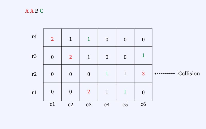
Retrieval
How do we retrieve the count of each element, given that each element can map to multiple locations in the hash table? We select the count that is least from the table. So, for element A, we select count two from row-1 and column-3. This is to ensure that we have the least approximation on the counter when we select the cell with the least counter.
The Count-Min Sketch data structure is a suitable replacement for the Hash Table, which can grow unbounded in memory. However, we will still keep a heap to keep a list of topK elements.
High-level Architecture
Before we go through each of the components in detail, let us first discuss the higher-level data flow for the system. We will discuss the system's design with two design goals in mind.
Design Goal #1: A fast system (gets results within seconds) — the results are approximate.
Design Goal #2: A relatively slower system (gets results within minutes to hours) — the results are accurate.
It is worth noting to discuss this question with the interviewer and understand whether they would be interested in design goal #1 or design goal #2 or both. You can then discuss designs based on what the interviewer is looking for.
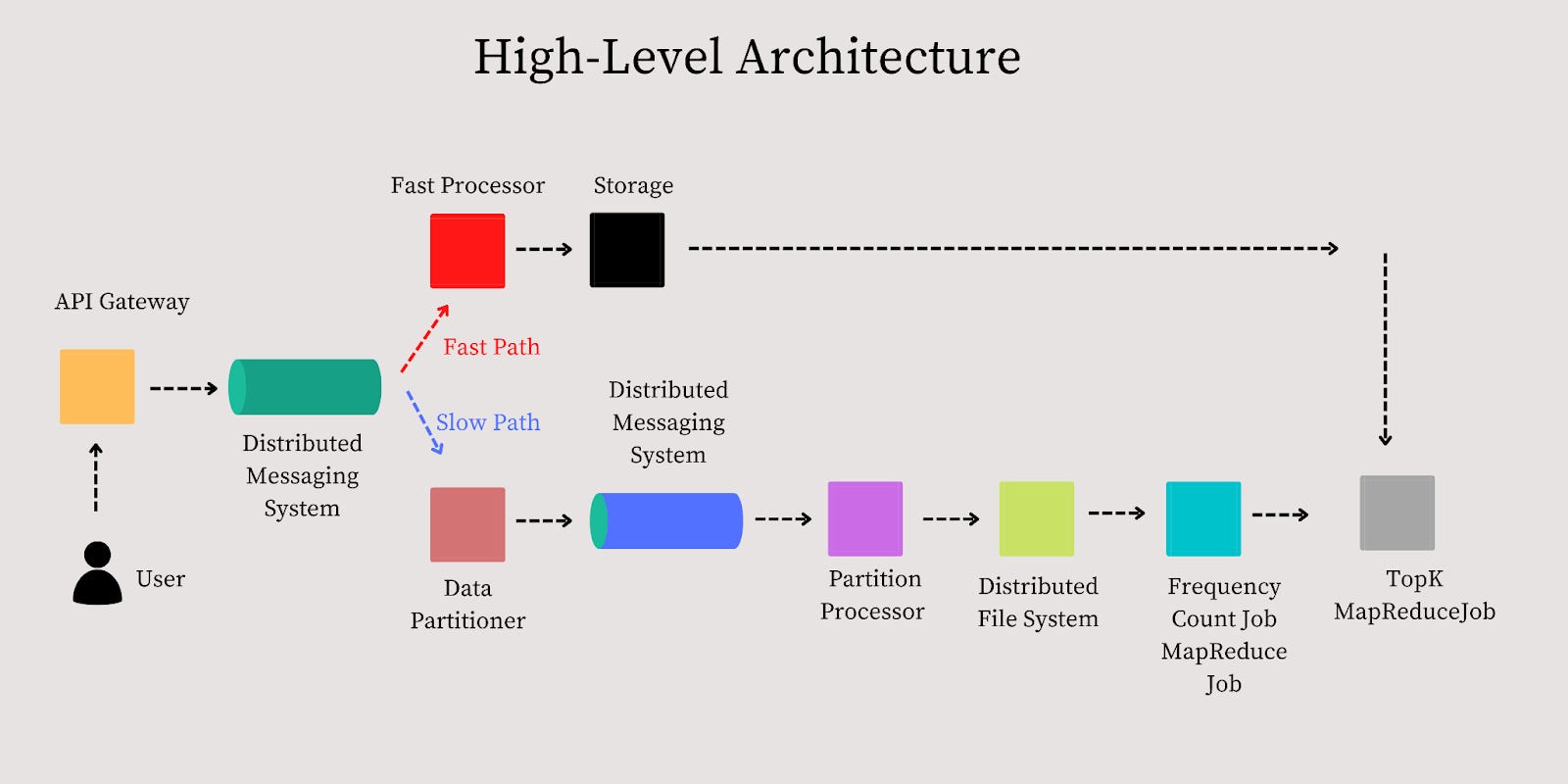
Higher-level Data Flow
Before we go any further, let us discuss the higher-level data flow, and then we can discuss the details of each of the components.
API Gateway
An essential function of an API Gateway is to route the request from the client to the backend services. In the modern tech stacks, most distributed systems use API gateways in the distributed systems. We are interested in using the API Gateway to look at the request logs for our use case. The request logs contain information about which a user viewed a video. The API Gateway is designed as follows:
The single entry point for all clients.
Aggregates data on the fly or via a background process the processes logs. Data is flushed based on either time or size. A bounded-sized memory buffer is used in the API Gateway to map each request to a count. It can be implemented using a Hash-Table, as discussed in this blog post. Once the buffer becomes full, the data is flushed onto a disk.
Last but not least, the data is serialized in a compact binary format (e.g., Apache Avro) to bring efficiency. This is done to ensure that the size of the data transferred over the network is compacted and bandwidth utilization is low.
Distributed Messaging System
The data is then sent to a distributed messaging queue such as Apache Kafka or AWS Kinesis. Internally, we do not have any specific preference for a partitioning scheme for the scope of this problem. A random partitioning scheme will serve the purpose of distributing data across different nodes within the cluster.
Fast Path
We will calculate an approximate list of heavy hitters on the fast path and ensure that the result is available within seconds.
Fast Processor
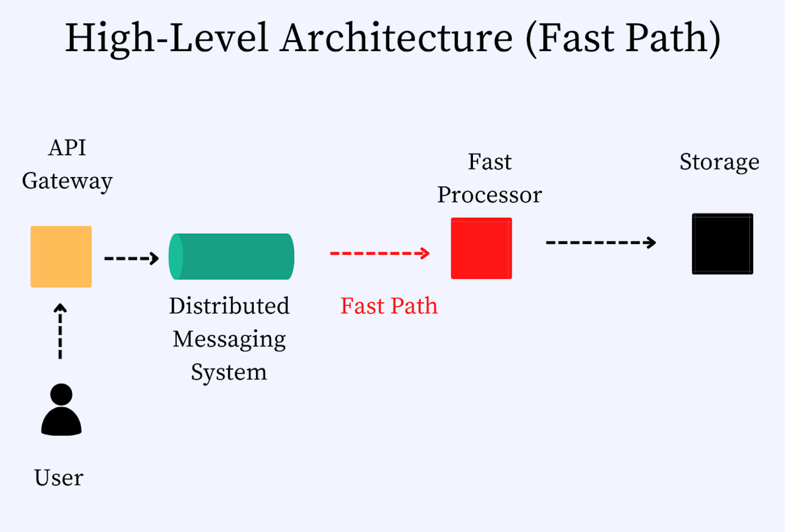
The first component on the fast path is a service called the fast processor. It creates a count-min sketch and aggregates data for a short period (seconds). Because memory is no longer a problem, there is no need to partition. To ensure that the system remains highly available (one of the requirements of the system’s design), we need to ensure that the data is replicated. Otherwise, the system may not remain available when one of the processor nodes shuts down. However, we have the Slow Path as a backup to the Fast Path so that it may be an acceptable tradeoff. It is good to discuss this as a tradeoff with the interviewer and understand the requirements clearly.
Storage
Every several seconds the fast processor flushes data to a secondary storage layer. It is good to note that the count-min sketch data structure has a predefined size in memory. The memory requirements do not grow unbounded within the fast processor. So, we could keep the count of the videos views for a more extended period in memory in the fast processor. However, the drawbacks of keeping the data in memory for a long time are as follows:
The higher the time window for which the data is not persisted on the secondary storage, the higher the probability of it being lost.
The longer the data remains in memory, the longer it takes to calculate the final results.
The storage layer can be built using SQL or NoSQL database schemes. In my opinion, both could work. It builds the final count-min sketch and stores a list of top k elements for a period of time. Given this layer ensures that the data remains durable and highly available, data replication is required.
Slow Path
We will calculate a precise list of heavy hitters, and the result will be
available within minutes or hours, depending on the data volume. Given that our objective is to calculate an accurate answer to the problem, we will dump the data on the disk and then use one of the following options to calculate the topK heavy hitters. Let us go through the options and explore their pros and cons.
Option #1: Use MapReduce
To implement MapReduce, we can dump the data onto a distributed storage layer such as HDFS or S3. We can then run two different MapReduce jobs.
Job #1: Count the frequency of each item (view of a YouTube video).
Job #2: Calculate the TopK hitters.
Pros: Produce accurate results.
Cons: MapReduce tends to be slow.
Option #2: Use Data Partitioner And Map Reduce
Step 1#: Using A Data Partitioner
The data partitioner reads batches of events from the Distributed Messaging Queue and partitions them into individual events. The partitioner will use a key derived from the video identifier and time window to hash the keys into different partitions.
Each partition is then sent to different partitions of a messaging queue. The messaging queue can be Apache Kafka, AWS Kinesis, or any other queuing system supporting distributed processing.
It is also worth noting that the data partitioner should take care of hot partitions. If a particular set of videos are being watched heavily, the partitioner will need to rebalance the data flowing into the stream for the specific data partition. This may be done by creating a duplicate partition for the hot set of keys or using a different hashing scheme.
Step #2: Using A Distributed Messaging Queue
Depending on our platform, each partition sent to the messaging queue will be sharded in Kafka or Kinesis. To ensure availability, both Kafka and Kinesis take care of data replication if one of the shards becomes unavailable.
Step #3: Partition Processor
Next, we need a component to read each partition and aggregate it further. Let us call this component a partition processor. The main job of the partition processor is to aggregate the partitioned data in memory over several minutes and generate the data in predefined file sizes and store it in the distributed file system.
Data Flow: Fast Path
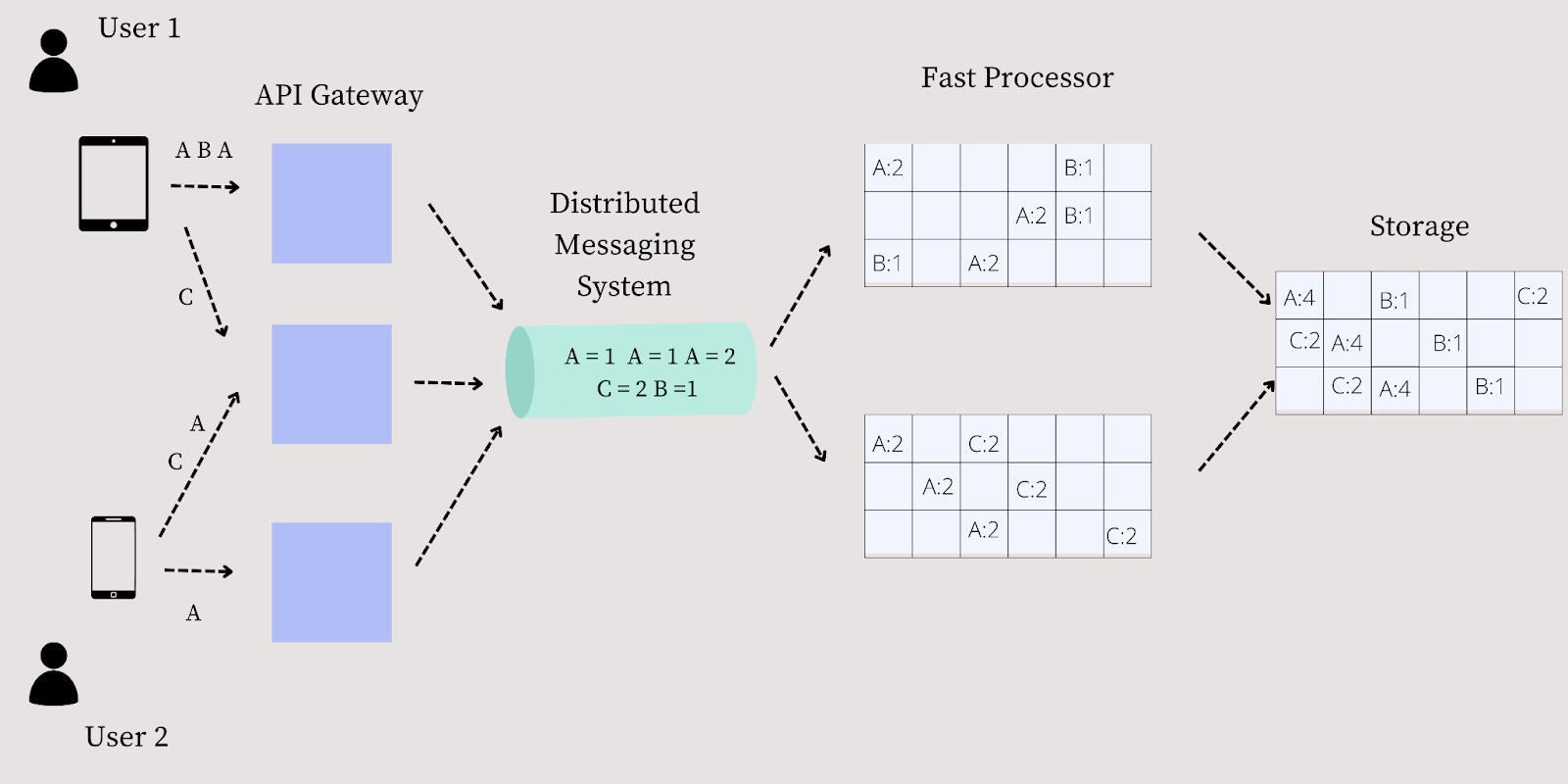
Let us look at the data flow of the system in detail. Refer to the figure above to understand the flow better.
Step #1: Two different users, User 1 and User 2 view YouTube videos, A B A C, and A A-C, respectively.
Step #2: The views are distributed to the different API Gateways. Let us assume three API Gateways (G1, G2, and G3). The requests A B A from User 1 flow to G1. The requests from C from User 1 and A-C from User 2 flow to G2. The request A from User 2 flows to G2.
Step #3: The API Gateways log the requests, and the logs are forwarded to the Distributed Messaging Queue. The Messaging Queue then forwards the requests to the two different fast processors.
Step #4: The fast processors then use the min-sketch data structure to create a view of the video hits. Fast Processor 1 would get the following aggregated results A:2 and B:1, and Fast Processor 2 would get A:2 and C:2.
Step #5: The fast processors then take the top K and pass it to the storage. Assume that k is 2. The storage then aggregates the two outputs and creates a single view to find the top K elements. The result would be A:4 and C:2.
Note the assumption here is that the data is not lost in between due to collisions. However, the results may be approximate in the real world but within an error bound.
Data Flow, Slow Path
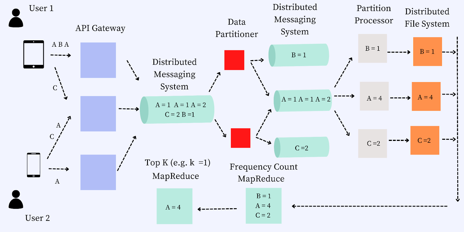
Let us walk through the data flow for the slow path. The steps for the data flow are as follows:
Step #1: Two different users, User 1 and User 2 view YouTube videos, A B A C, and A A C, respectively.
Step #2: The views are distributed to the different API Gateways. Let us assume three API Gateways (G1, G2, and G3). The requests A B A from User 1 flow to G1. The requests from C from User 1 and A-C from User 2 flow to G2. The request A from User 2 flows to G2.
Step #3: The distributed messaging queue then forwards the data to a data partitioner. The data partitioner partitions the data and passes it to a data messaging system.
Step #4: The data messaging system picks up each partition and passes it to the appropriate partition processor. The goal of the partition processor is to aggregate the data for each partition and aggregate the views.
Step #5: The partition processor dumps the data into a distributed file system to calculate the topK elements.
Step #6: A mapper is then used to count the frequency of each of the partitions on the distributed file system.
Step #7: A reducer is used to reduce and find the topK elements.
It may not be clear how and why we need the MapReduce jobs as we haven’t discussed those in detail. Let us discuss those in detail in the next section.
MapReduce Jobs
We use two jobs for calculating the TopK Heavy Hitters. These are Frequency Count MapReduce and TopK MapReduce. Let us discuss each of these in detail in the following section.
Frequency Count MapReduce
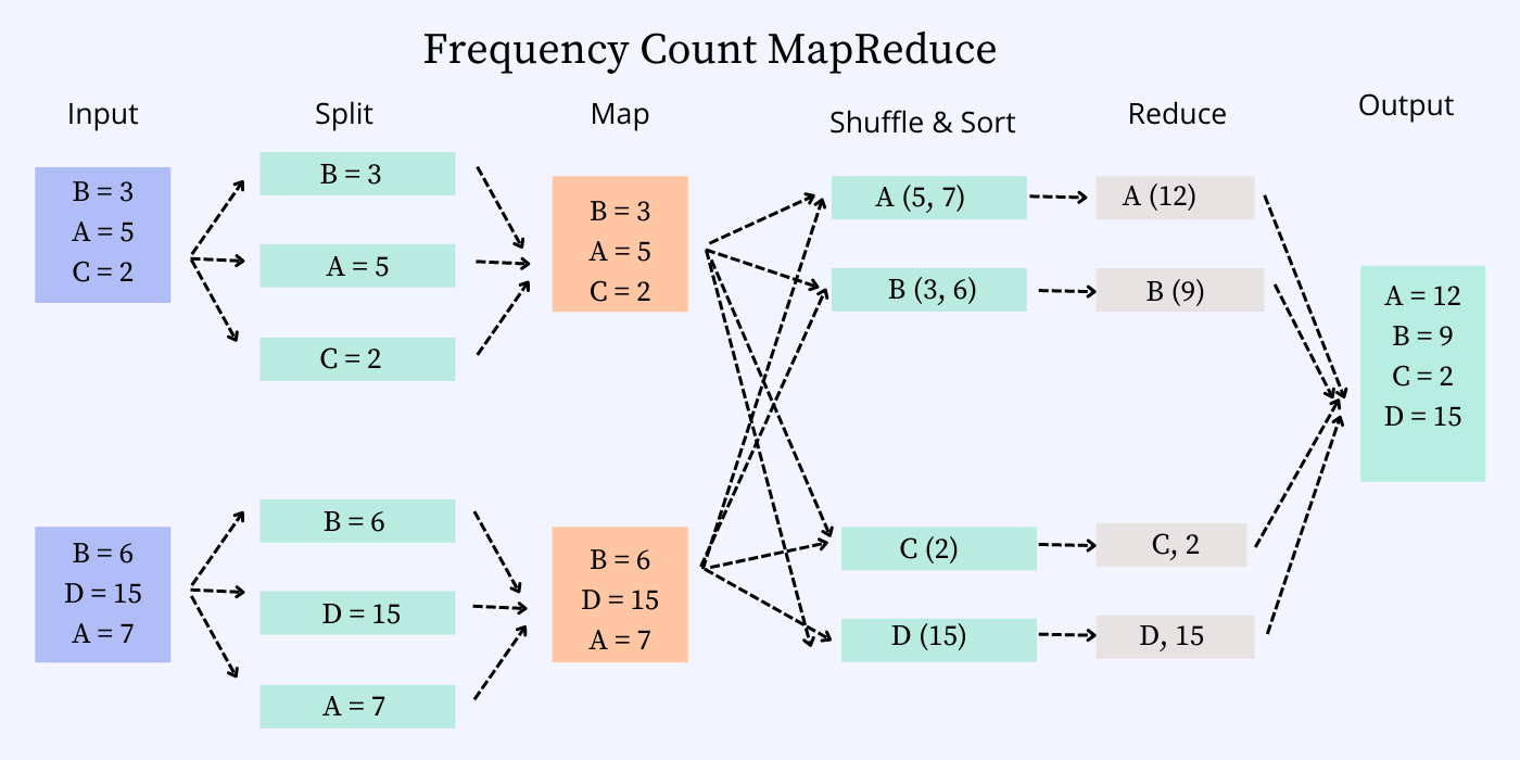
Let us discuss the steps involved in the mapper job for the frequency count job.
Stage #1: The input is split into individual records from the input files read from the distributed storage (HDFS, S3).
Stage #2: Each of the individual records is then mapped into partitions for aggregate on those partitions by a mapper job.
Stage #3: The mapper’s output is then shuffled by the key and combined in the same partition.
Stage #4: The reducer then aggregates each key and emits the count for each key.
Stage #5: The output file is generated by aggregating all the keys in one place. The Reducer job uses this output.
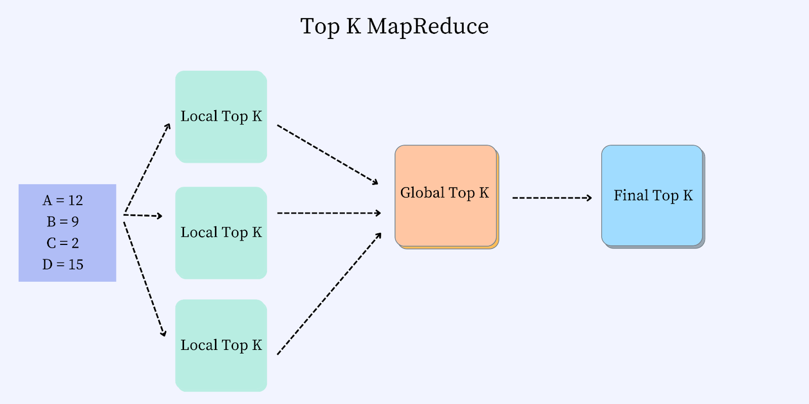
TopK MapReduce
The different stages for the TopK MapReduce are as follows:
Stage #1: The input from FrequencyCount MapReduce is partitioned, and the TopK is calculated over each partition in the map stage.
Stage #2: The topK from each partition is aggregated into a single node, and a global TopK is emitted in the reduce stage.
This wraps up the overall discussion of the problem. I hope you found the discussion helpful.
Hey Ravi, I like the way you are converting Mikhail Smarshchok's youtube videos to blog posts. You should be putting an appreciation note mentioning his efforts in the blog somewhere.
Hi Ravi, thanks for sharing this insightful blog.
One question:
Computing global top k elements using local top k elements might not be always correct.
eg.
Suppose we are interested in top 2 elements and local frequency count is as below,
Local1 = A:8, B:7, C:6
Local2 = A:3, B:2, C:6
Top 2 from local1 is A, B and from local2 is C,A
Global top 2 will be A:11, B:7
But it should be C:12, A:11.
Please let me know what exactly i am missing here. Thanks